By Yingqi Zhao, Ph.D
Major Work:
1. optimal treatment rule $$d^*$$ can be estimated within a weighted classification framework, with weights determined from the clinical otucomes.
2. Replace 0-1 loss with convex surrogate loss with SVM via hinge loss
hinge loss function image
3. OWL approach beeter select targeted therapy while making full use of available information
Paper Structure
Sec 2: math for ITR, then formulate it as OWL; weighted SVM approach for optimal ITR
Sec 3: consistency and risk bound results; Faster convergence rates can be achieved with additional marginal assumptions on the data generating distribution
Sec 4: Simulation to evaluate performance
Sec 5: real data Nefazodone-CBASP
Appendix: proofs of theoretical results
Method
Two arms randomized trial (intervention vs control), action $$A\in {-1, 1}$$, independent of patients' prognostic var $$X=(X_1, ..., X_d)^T \in \chi$$.
Assume reward $$R$$ is bounded and larger the better.
ITR denote as $$D$$: a map from space of prognostic $$\chi$$ to space of treatments, $$A$$.
Optimal ITR: a rule that maximized the expected reward if implemented
Outcome Weighted Learning (OWL) for Estimating Optimal ITR: non parametric approach which directly maximizes the value function based on an outcome weighted learning method
Denotation, Assumption & Lemma
- $$P$$: distribution of $$(X,A,R)$$; with expectation $$E$$
- $$P^D$$: distribution of $$(X,A,R)$$ given that $$A=D(X)$$; with expectation $$E^D$$
- Assumption: $$P(A=a)>0$$ for $$a=1$$ and $$-1$$, which means both actions is not impossible
- $$\frac{dP^D}{dP}=I(a=D(x))/P(A=a)$$ (a version of the Radon-Nikodym derivative)
- $$D(x)$$ can always be represented as $$sign(f(x))$$ for some decision function $$f$$.
- Linear Decision Rule: $$f(X)=<\beta,x>+\beta_0$$; ITR assign X into treatment 1 if $$f(X)>0$$ ; Define $$||f||$$ as Euclidean norm of $$\beta$$; introduce $$\xi_i$$ as slack variable for subject $$i$$ to allow a small portion of wrong classification. $$C>0$$ as classifier margin.
- Any function $$f(\cdot)$$ in $$H_k$$ takes the form $$\sum_{i=1}^m\alpha_ik(\cdot, x_i)$$
- Estimated value function given any ITR $$D$$ is $$P^* _n[I(A=D(X))R/P(A)]/P^* _n[I(A=D(X))/P(A)]$$, where $$P^*_n$$ denotes the empirical average using the validation data and $$P(A)$$ is the probability of being assigned treatment $$A$$.
Equations
Value function associated with $$D$$
where $$P^D$$ is the CDF under decision rule $$D$$ and $$P$$ is CDF under general case; $$\pi=P(A=1)$$
Note that $$D^*$$ does not change if $$R$$ replaced by $$R+c$$, we can just assume $$R$$ is nonnegative.
Finding $$D*$$ to maximize $$V(D)$$ is equivalent to minimize weighted classification error (weigh each misclassification event by $$R/(A\pi+(1-A)/2))$$.
Find a convex surrogate loss for the 0-1 loss, one of the most popular is the hinge loss used in the SVM, and also penalize the complexity of the decision function to avoid overfitting
where $$x^+=max(x,0)$$ and $$||f||$$ is some norm for $$f$$. We cast the problem of estimating the optimal ITR into a weighted classification problem using SVM.
The Linear Decision Rule has equivalent expression for objective function above:
subject to $$A_i(<\beta,X_i> + \beta_0) \ge (1-\xi_i),\ \xi_i \ge0$$ and $$\kappa>0$$ is a tuning parameter, $$R_i/\pi_i$$ is the weight for $$i$$th point.
We can then introduce Lagrange Multiplier and obtain
\alpha_i\{A_i(<\beta,X_i> + \beta_0)-(1-\xi_i)\}-\sum_{i=1}^n\mu_i\xi_i
where $$\alpha_i\ge0,\mu_i\ge0$$
After taking derivatives and plug equations into the Lagrange function, obtain the dual problem
subject to $$0\le\alpha _i \le\kappa _i/\pi_i,\ i=1,... ,n$$ and $$sum _{i=1}^n\alpha_i A_i=0$$
Soln:
and $$\hat{\beta}_0$$ can be solved using margin points $$(0 < \hat{\alpha}_i, \hat{\xi}_i=0)$$ subject to the KKT conditions. *(P421, Hastie, Tibshirani & Friedman 2009)*.
Decision Rule: Given by $$sign(<\hat{\beta}, X> + \hat{\beta}_0)$$.
Nonlinear Decision Rule
let $$k: \chi * \chi \to R$$ (Kernel function) be continuous, symmetric and positive semidefinite.
Given a real-valued kernel function k, we can associate with it a reproducing kernel Hilbert space (RKHS) $$H_k$$, which is completion of the linear span of all functions $${k(\cdot, x), x\in \chi}$$
We also define the norm in $$H_k$$, $$||...||_k$$ as
for $$f(\cdot)=\sum_{i=1}^m\alpha_ik(\cdot, x_i)$$ and $$g(\cdot)=\sum_{i=1}^m\beta_jk(\cdot, x_j)$$
Optimal Decision function
where $$(\hat\alpha_1, ..., \hat\alpha_n)$$ sovles
subject to $$0\le \alpha_i \le \kappa R_i/\pi_i,\ i=1,..., n$$ and $$\sum_{i=1}^n\alpha_i A_i=0$$.
Simulation
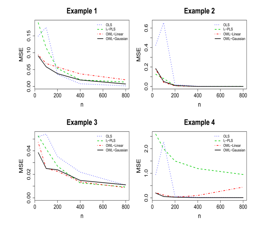
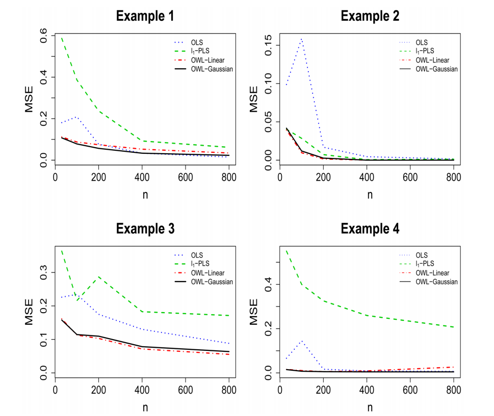
50-dimensional vectors of prognostic variables $$X_1, ..., X_{50}$$, consisting of independent $$U[-1, 1]$$ variates. Treatment $$A$$ is generated from $${-1, 1}$$ independently of $$X$$ with $$p(A=1)=1/2$$. Response $$R$$ is normally distributed with mean $$Q_0 = 1+2X_1 +X_2 + 0.5 X_3 + T_0(X,A)$$ and standard deviation $$1$$. $$T_0(X,A)$$ reflects the interatction between treatment and prognostic variables and si chosen to vary according to the 4 differnet scenarios.
The decision boundaries in the first three scenarios are determined by X 1 and X 2 . Scenario 1
corresponds to a linear decision boundary in truth, where the shape of the boundary in
Scenario 2 is a parabola. The third is a ring example, where the patients on the ring are
assigned to one treatment, and another if inside or outside the ring. The decision boundary in
the fourth example is fairly nonlinear in covariates, depending on covariates other than X 1
and X 2 . For each scenario, we estimate the optimal ITR by applying OWL.
Gaussian Kernel in weighted SVM algorithms
Tuning parameters: $$\lambda_n$$ the parameter for penalty and $$\sigma_n$$ the inverse bandwidth of the kernel.
Note that $$\lambda_n$$ plays a role in controlling the severity of the penalty on the functions and $$\sigma_n$$ determines the complexity of the function class utilized, $$\sigma_n$$ should be chosen adaptively from the data simulataneously with $$\lambda_n$$. (In example of linear decision boundary, larger $$\lambda_n$$ generally coupled with smaller $$\sigma_n$$ for equivalent value function levels.)
Compare 4 Methods
- the proposed OWL using Gaussian kernel (OWL-Gaussian)
- the proposed OWL using linear kernel (OWL-Linear)
- the l 1 penalized least squares method ( l 1 -PLS) developed by Qian & Murphy (2011), which approximates E ( R | X , A ) using the basis function set (1, X , A , XA ) and applies the LASSO method for variable selection
- ordinary least squares method (OLS), which estimates the conditional mean response using the same basis function set as in 3 but without variable selection
The last two approaches estimate the optimal ITR using the sign of the difference between the predicted
E ( R | X , A = 1) and the predicted E ( R | X , A = −1).
Validate with 2 Criteria
- evaluate the value function using the estimated optimal ITR when applying to an independent and large validation data
- evaluate the misclassification rates of the estimated optimal ITR from the true optimal ITR using the validation data
a validation set with 10000 observations is simulated to assess the performance of the approaches
Simulation Results
- Simulations show there are no large differences in the performance if we replace the Gaussian kernel with the linear kernel in the OWL
- under certain circumstances, it is useful to have a flexible nonparametric estimation procedure to identify the optimal ITR for the underlying nonparametric structures
- the OWL with either Gaussian kernel or linear kernel has better performance, especially for small samples, than the other two methods, from the points of view of producing larger value functions, smaller misclassification rates, and lower variability of the value function estimates (n = 200 is the breaking point)
Under 4 different scenario, MSE for Value Functions of ITR
Under 4 different scenario, MSE for Misclassification Rate of ITR
- OWL procedure outperform a traditional logistic regression
- Numerical results indicate that $$log_2\sigma_n$$ is linear in $$log_2\lambda_n$$ and the ratio between teh slopes is close to the reciprocal ratio between teh dimensions of the covariate spaces.
Real Data Analysis
To estimate the optimal ITR, we perform pairwise comparisons between all combinations of
two treatment arms, and, for each two-arm comparison, we apply the OWL approach.
The score on the 24-item Hamilton Rating Scale for Depression (HRSD) was
the primary outcome, where higher scores indicate more severe depression.
Rewards used in the analyses are reversed HRSD scores and the
prognostic variables X consist of 50 pretreatment variables. The results based on OWL are
compared to results obtained using the l 1 -PLS and OLS methods which use (1, X , A , XA ) in
their regression models.
Real Data Performance
- Altough l1-PLS and OWL is relatively the same and both better than the OLS, l1-PLS endures a large variability concerning recommending treatment for patients during cross validation (split into 5 equally sized groups)
- OWL not only yields ITRs with the best clinical outcomes, but the ITRs also have lowest variability compared to the other methods.
Leave A Comment