3 or more Hidden Layer then you have a deep network
Activation Function
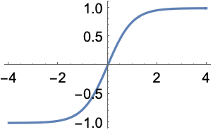
Hyperbolic Tangent: $$tanh(z)$$, where $$z = wx+b$$
The graph looks like this
Rectified Linear Unit(ReLU): relatively simple function: max(0, z)
Cost Function
Quadratic Cost $$C = \sum(y-a)^2/n$$, where $$a$$ is the activation value
Unfortunately this quadratic calculation can cause a slowdown in learning speed, instead we use
Cross Entropy allows for faster learning (because the larger the difference between y and a, the faster the neuron can learn)
Back Propagation
Used to calculate the error contribution of each neuron after a batch of data is processed; relies heavily on the chain rule to go back through the network and calculate these errors.
Manual Creation of Neural Network
Operations: node and graph
Operation Class:
- INput Nodes
- Output Nodes
- Global Default Graph Variable
- Compute - Overwritten by extended classes
Tensorflow
TF Syntax Basic
CNN Convolutional Neural Network
Initialization of Weights Options
Xavior (Glorot) Initialization: Uniform/Normal
Draw weights from a distribution with 0 mean and specific variance for each neural
where $$W$$ is the distribution and $$n_{in}$$ is the number of input neuron to that specific neuron.
We have
where $$X$$ and $$Y$$ are independent.
And if we have both expectation of $$X_i$$ and $$W_i$$ as 0, then
And
where $$Var(W_i)=\frac{1}{n_{in}}$$ (more practical version) or $$Var(W_i)=\frac{2}{n_{in}+n_{out}}$$ (original formula)
Batch Size
Smaller --> less representative of data
Larger --> longer training time
Adjust Learning Rate Based off Rate of Descent
2nd order behavior of the gradient descent
- AdaGrad
- RMSProp
- Adam: allows that change to happen automatically
Vanishing Gradient: as you increase the number of layers in a network, the layers towards the input will be less affected by the error calculation occurring at the output as you go backwards through the network.Initialization and Normalization help mitigate these issues.
Overfitting: use dropout (unique to neural networks) to remove neurons during training randomly, so that network doesn't over rely on any particular neuron.
MNIST
We can think of the entire group of 55000 images as a tensor (an n-dimensional array)
For the labels, we'll use One-Hot Encoding, the label is represented based off the index position in teh label array; the corresponding label will be a $$1$$ at the index location and $$0$$ everywhere else.
Eventually, the training set would be (28 * 28) * 55000 = 784 * 55000 and labels for the training data ends up being large 2-D array (10, 55000)
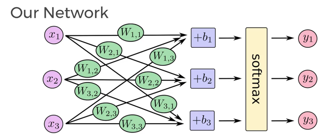
Softmax Regression
Returns a list of values between 0 and 1 that add up to 1, use this as a list of probabilities!
for $$j=1,...,K$$.
We use Softmax as our activation function
and
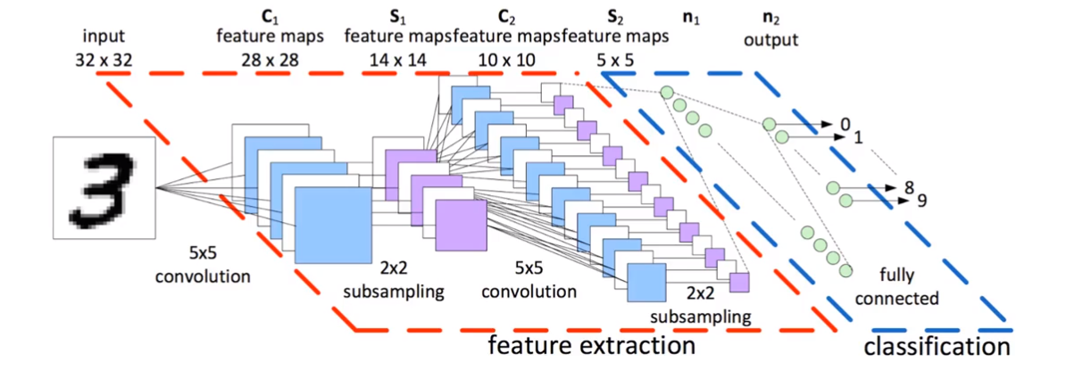
Convolutional Neural Network
For MNIST dataset, we have 4 dimensional sensors, (I, H, W, C)
- I: images
- H: height of image in Pixels
- W: width of Image in Pixels
- C: color channels: 1-grayscale, 3-RGB
CNN Structure: each unit is connected to a smaller number of nearby units in next layer -> this can resolve the problem of images been too big (256 * 256) and that too many parameters
Features
- Each CNN layer looks at an increasingly larger part of the image
- Having units only connected to nearyby units also aids in invariance.
- CNN also helps with regularization, limiting the search of weights to the size of the convolution.
Padding: when reach the edge of image, we add a "padding" of zeros around the image.
Filter Size and Stride
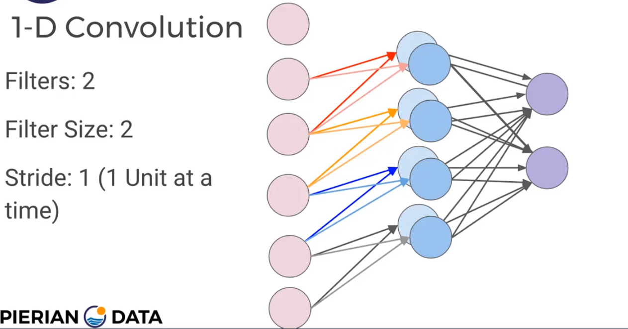
Add another set of neurons ready to accept another set of weights/filter; Each filter is detecting a different feature.
Stride means how fast you move along the image with your filters. 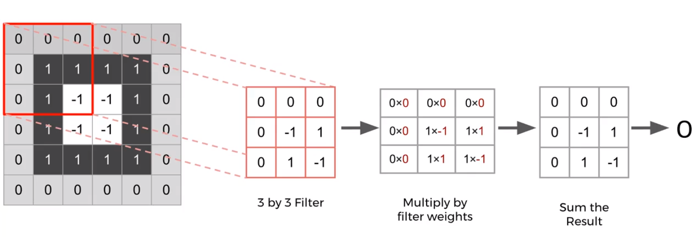
Pooling layers: subsample the input image, which reduces the memory use and computer load as well as reducing the number of parameters.
Basically for example we evalute the 2-by-2 maximum value
Dropout: form of regularization to help prevent overfitting
Leave A Comment