Date: 2017/04/16
source: http://math.usu.edu/jrstevens/stat5570/2.3.Clustering.pdf
# Heatmap Trial
library(cluster)
library(RColorBrewer)
set.seed(123)
x1 <- c(rnorm(20,sd=.05),
        rnorm(20,mean=1,sd=.05),
        rnorm(20,mean=1.5,sd=.05))
x2 <- 4+c(rnorm(20,sd=2),
          rnorm(20,mean=8,sd=1.5),
          rnorm(20,mean=8,sd=1))
x1.sc <- x1/sd(x1)
x2.sc <- x2/sd(x2)
hmcol <- colorRampPalette(brewer.pal(10,"RdBu"))(256)
csc <- c(hmcol[50],hmcol[200]) # define side colors
heatmap(cbind(x1.sc,x2.sc),scale="column",col=hmcol,
        ColSideColors=csc,cexCol=1.5,cexRow=.5)

# ---- try with ALL datasets
source("http://bioconductor.org/biocLite.R")
biocLite(c('affy', 'ALL')) # download packages

library(affy); library(ALL); data(ALL)
gn <- featureNames(ALL) # ALL is an ExpressionSet object
# Choose a subset of genes (How in Unit 3)
gn.list <- c("37039_at","41609_at","33238_at","37344_at",
             "33039_at","41723_s_at","38949_at","35016_at",
             "38319_at","36117_at")
t <- is.element(gn,gn.list) # decide whether contained in gn.list
small.eset <- exprs(ALL)[t,c(81:110)]
# Define color scheme
hmcol <- colorRampPalette(brewer.pal(10,"RdBu"))(256)
## Columns
# Here, the first 15 are B-cell patients; rest are T-cell
cell <- c(rep('B',15),rep('T',15))
csc <- rep(hmcol[50],ncol(small.eset))
csc[cell=='B'] <- hmcol[200]
colnames(small.eset) <- cell
## Rows
rownames(small.eset)
# [1] "33039_at" "33238_at" "35016_at" "36117_at"
# [5] "37039_at" "37344_at" "38319_at" "38949_at”
# [9] "41609_at" "41723_s_at"
## (Could add rsc [row-side colors] similar to csc
## if we knew functional differences among genes)
## Make heatmap
heatmap(small.eset,scale="row",col=hmcol, ColSideColors=csc)

# ---- enhanced heatmap
# Look at 'enhanced' heatmap
### The white dashed lines show the average for each column
### (on the left-to-right scale of the key),
## whereas the white solid lines show the deviations from
## the average within arrays.
library(gplots)
heatmap.2(small.eset, col=hmcol, scale="row",
          margin = c(5,5), cexRow= 0.8,
          # level trace
          tracecol='white',
          # color key and density info
          key = TRUE, keysize = 1.5, density="density",
          # manually accentuate blocks
          colsep=c(15), rowsep=c(5,6,7), sepcolor='black')

# ---- Heamap Alternative use
# Alternative use for heat maps
# 1 Visualize distance between arrays
# 2 recall defining distance between genes and between arrays --> get distance matrix
# 3 run heatmap on distance matrix --> often called false color image
# source("http://bioconductor.org/biocLite.R")
# biocLite('bioDist')
library(bioDist)
d.gene.cor <- cor.dist(small.eset)
heatmap(as.matrix(d.gene.cor),sym=TRUE,col=hmcol,
main='Between-gene distances (Pearson)',
xlab='probe set id',labCol=NA)
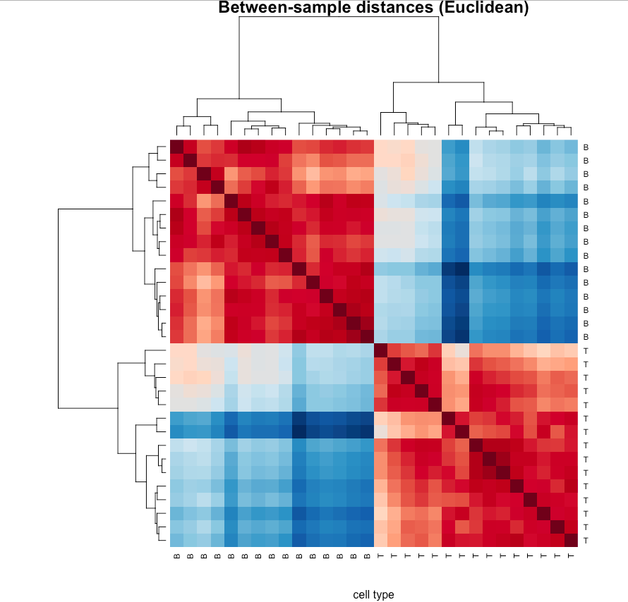
d.sample.euc <- euc(t(small.eset))
heatmap(as.matrix(d.sample.euc),sym=TRUE,col=hmcol,
main='Between-sample distances (Euclidean)',
xlab='cell type')
# A poor color scheme (like red/green) could prevent a large percentage of the
# audience from gaining any information from the visualization.
# (deuteranopia) 红绿色盲
# Consider alternative color scheme
red.hmcol <- colorRampPalette(brewer.pal(9,"Reds"))(256)
green.hmcol <- colorRampPalette(brewer.pal(9,"Greens"))(256)
use.hmcol <- c(rev(red.hmcol),green.hmcol)
heatmap(as.matrix(d.sample.euc),sym=TRUE,col=use.hmcol,
main='Alternative Color Scheme',xlab='cell type')
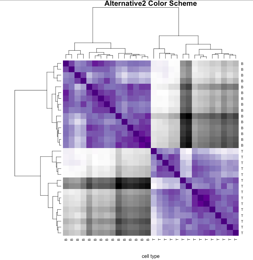
red.hmcol <- colorRampPalette(brewer.pal(9,"Purples"))(256)
green.hmcol <- colorRampPalette(brewer.pal(9,"Greys"))(256)
use.hmcol <- c(rev(red.hmcol),green.hmcol)
heatmap(as.matrix(d.sample.euc),sym=TRUE,col=use.hmcol,
main='Alternative2 Color Scheme',xlab='cell type')
# Median split silhouette (MSS) -- find small clusters in big cluster
# Hierarchical Ordered Partitioning And Collapsing Hybrid
# Bootstrapping HOPACH in R
# please check http://math.usu.edu/jrstevens/stat5570/2.3.Clustering.pdf
# more image instrctive material about clustering methods, check
# http://compbio.uthsc.edu/microarray/lecture1.htm
Leave A Comment