 + Solo Top10 Predictive Model in RShiny")
Project Description
Data Srouce & Discription
Huge thanks to KP who is both a PUBG player and web scrapper master. He used his own PUBG account as initial seed and expand the players network by collecting data of all players that he encountered and those encountered players he encountered...
The original data is gathered by pubg.op.gg game tracker website where you can view your PUBG ranking, weapon analysis, population distribution and information map.
The 20.3 GB dataset I used is from Kaggle created by KP. It provides two zips: aggregate and deaths.
- In deaths, the files record every death that occurred within the 720k matches. That is, each row documents an event where a player has died in the match.
- In aggregate, each match's meta information and player statistics are summarized (as provided by pubg). It includes various aggregate statistics such as player kills, damage, distance walked, etc as well as metadata on the match itself such as queue size, fpp/tpp, date, etc.
For detailed information about dataset and variable columns, please visit Kaggle website.
Interpreting Positional Data:
The X,Y coordinates are all in in-game coordinates and need to be linearly scaled to be plotted on square erangel and miramar maps. The coordinate min,max are 0,800000 respectively.
Potential Bias in the Data (by dataset author):
"The scraping methodology first starts with an initial seed player, I chose this to be my own account (a rather low rank individual). I then use the seed player to scrape for all players that it has encountered in its historical matches. I then take a random subset of 5000 players from this and then scrape for their historical games for the final dataset. What this could produce is an unrepresentative sample of all games played as it is more likely that I queued and matched with lower rated players and those players more than likely also got matched against lower rated players as well. Thus, the matches and deaths are more representative of lower tier gameplay but given the simplicity of the dataset, this shouldn't be an issue."
Data Import & Guidance
In order to deal with the entire PUBG dataset, I choose MySQL server in Ubuntu. If you don't have a MySQL server installed in your machine yet, go google and there are lots of good tutorial to teach you how to install with sudo apt-get install and you can start from there. What I want to share is how to avoid not enough root space error on your machine (which is painful) and how to import a bunch of csv files into your MySQL. Since this part is more of an engineering work, I'll leave you to my corresponding code portfolio page Code for PUBG Data Analysis and my trash talk blog [How MySQL Ruined My Day (even AWS didn't save it)]( "How mySQL Ruined My Day (even AWS didn't save it)").
Now assume you are done with data import, you have 2 really big table in your PUBG database. DON'T TRY TO DO ANYTHING WITH THEM YET! Given such large table even a select count(*) from meta will take like a year to finish. What you would like to do here is to skip out and think:
- What is my data analysis objective?
- What types of variables do I need?
- How large a dataset can satisfy my analysis goal?
Normally you already knew what you want to get from this dataset; so now take your time and inspect all the variables -- mark those you want to include and exclude; create new ones to better suit your analysis.
After that, you want answers to these questions: Can I narrow down my dataset? In order to perform meaningful statistical results how many data do I need? (In our case, how many players do I need to obtain a rather stable population distribution description?) 8 of out 10 times you will say YES to these questions, and the next thing you'll do is data preparation (filtering, sorting, grouping, etc.).
Objective & Questions
Here in my report, I'd like to consider these following questions:
- What is the PUBG player statistics in my dataset? (longitudinal trend, distribution, etc.)
- On average, how many player do we eliminate before making Top10?
- Can we predict Top10 based on player statistics?
Data Preparation
Anything related to coding and scripts are posted on Code for PUBG Data Analysis
In order to answer the questions above, first I need to create a new table with players meta information such as avg_kills and average_walk_dist. My instinct tells me that I do not need that many player records, hence I want to look at select count(player_name) from meta; which is how many games in total does a player played in our study population?
I don't know whether MySQL will be of high performance on filtering, but I used a Hadoop Map-reducer-like parallel mclapply() function in R, which proves to be very effective with select count(*) from meta statement.
We first look at players count barplot who played from 1 to 50 games in total.

We can notice from the histogram that there are many players who only played PUBG for once! They just don't know how enjoyable PUBG is~ In order to come up with a reasonable threshold for the Number of Times Playing PUBG, I use following calculation:
Assume that average play time for one match in PUBG is 20 min (reasonable), and one player needs about 10 hours to be familiar with the keyboards and sensitivity settings (works for me), so the average time a player reach his/her first performance plateau is after 30 matches -- and we'll use this to exclude those players who either don't play very often or quit the game very soon.
Again the R mclapply() function does a great help in filtering and summarizing the whole dataset for me. If you're interested in how I managed to clean up the whole dataset in about an hour, please go to Code for PUBG Data Analysis and locate the same section.
I tried to use MySQL to do the same job at the begining, but it is just unbearably slow...
Below is my data tidying workflow:
For meta table (aggregate files)
- for each subfile, filter by select_name
- combine
For combat table (deaths files), we also need to compute the combat range info
- for each subfile, only select killer_name, killer_position_x, killer_position_y, map, match_id, victim_name, victim_position_x, victim_position_y
- filter by select_name and by killer_name != victim_name (don't consider suicides)
- filter by neither the (killer_position_x, killer_position_y) nor (victim_position_x, victim_position_y) is (0, 0) (see: https://www.kaggle.com/mithrillion/kill-distance-analysis for detailed reasons)
- mutate a new column as shoot_range, sqrt(x^2 + y^2), drop coordinate var
- combine
- group by match_id, map and killer_name, summarise as avg_shoot_range, max_shoot_range for each player per match
Inner join 2 tables by match_id and killer_name
agg_df <- meta %>%
inner_join(combat_range, by = c("match_id", "player_name" = "killer_name"))
Eventually, I obtain the agg_df dataset, which contains a rather complete match information for 484679 PUBG players in 720607 matches with 12625083 (~12.6 million) records, each corresponds to statistics for a single player in a single game match.
> agg_df
# A tibble: 12,867,413 x 18
   date      game_size match_id             match_mode party_size player_assists player_dbno player_dist_ride player_dist_walk player_dmg player_kills player_name
   <chr>         <int> <chr>                <chr>           <int>          <int>       <int>            <dbl>            <dbl>      <int>        <int> <chr>
 1 2017-11-…        37 2U4GBNA0YmnNZYkzjkf… tpp                 2              0           0             2619             2510        175            2 GeminiZZZ
 2 2017-11-…        37 2U4GBNA0YmnNZYkzjkf… tpp                 2              0           1                0             1450        101            1 SoSpicy
 3 2017-11-…        37 2U4GBNA0YmnNZYkzjkf… tpp                 2              0           1                0              129        215            2 GucciManeD…
 4 2017-11-…        37 2U4GBNA0YmnNZYkzjkf… tpp                 2              0           0             2419             2474         75            1 subzero3
 5 2017-11-…        37 2U4GBNA0YmnNZYkzjkf… tpp                 2              0           0             1278             3287         84            1 Chogo82
 6 2017-11-…        37 2U4GBNA0YmnNZYkzjkf… tpp                 2              0           0                0             1522        117            1 sigbo
 7 2017-11-…        37 2U4GBNA0YmnNZYkzjkf… tpp                 2              0           1                0             1079        100            1 Jerryxp
 8 2017-11-…        37 2U4GBNA0YmnNZYkzjkf… tpp                 2              1           1                0             2065        151            1 XombieMari…
 9 2017-11-…        37 2U4GBNA0YmnNZYkzjkf… tpp                 2              0           0                0             2076         17            1 Essaldun
10 2017-11-…        37 2U4GBNA0YmnNZYkzjkf… tpp                 2              0           1                0              538        124            1 KeyBoardSu…
# ... with 12,867,403 more rows, and 6 more variables: player_survive_time <dbl>, team_id <int>, team_placement <int>, map <chr>, avg_shoot_range <dbl>,
#   max_shoot_range <dbl>
Exploratory Data Analysis (Answer to Problem 1: Player Statistics)
All matches are in TPP (thrid person perspective) mode. First we'd like to visualize the trend of PUBG matches. The matches collected are between Oct 20 2017 to Jan 10 2018, covering the period of PUBG pre-release and full-release (full-release start from Dec 21 2017). Combining R and Tableau, I managed to visualize the growing trend of daily matches. From the upper figure where I compare the daily matches between 2 maps offered in PUBG, and notice that since the launch of new map MIRAMAR, in the first week it was the 1st choice for players, and after that 2 maps tied and share evenly the match numbers. From the lower figure I compare the party size number of daily matches. PUBG is mostly a team game and most of the time there should be a squad fighting side by side struggling to be to last one stand and enjoy the chicken dinner, and the pie chart indicates that about half of the total matches in the time span of our dataset is played in squads.
PC users can click here for interactive Tableau.

Besides daily matches, I am also concerned about daily active users (DAU) during this time period, hoping to find something similar or different.

Due to web scrappy reason, the part of data collected at the start or the end date might be incomplete, so I decide to remove both ends from the figure and only show the DAU curve from Oct 21 2017 to Jan 09 2018. I observe that after losing players for about 2 weeks, the launch of new map might seems to restore the popularity of PUBG, but the DAU curve tells us that it didn't actually attract more players when compared with the previous records.
And why is there a lowest point on Dec 21? Here is what I find:
OFFICIAL SCHEDULE of Server Down for Maintenance:
Start: Dec 20 4PM PST / Dec 21 1AM CET
End: Dec 20 11PM PST / Dec 21 8AM CET
"To ensure a successful and smooth launch, we have altered the PC 1.0 maintenance schedule. It will start 2 hours earlier but end at the same time as before. Thank you for your understanding," a message from Bluehole Inc explains.
Overall it's about 9 hours of maintainess time for players.
Website to track most same-time player numbers : https://steamcharts.com/app/578080#1y
Relative background information:
"PlayerUnknown's Battlegrounds" is the most popular game of 2017. It has sold over 24 million copies and has boasted 3 million concurrent online players on the Steam gaming platform — and the full game isn't even technically out yet. "PUBG" has been in "early access" since it was made available to play in March.Early-access games are usually unfinished, and it's a stage in a game's development when players can get a taste for the game with the understanding that they can run into bugs and unfinished features. But the early-access version of "PUBG" was clearly good enough.
Next I'd like to plot the distribution of the other numeric variables in the dataset, sectioned by Party Size (Blue for Squad, Green for Duo and Red for Solo), and we'll briefly go over some variables to explain why they have such distribution.

- player_dbno shows the distribution of players knocking down without killing on other players. The first columns has a large proportion of red because for Solo, there are no such knocking down part, so all of the solo match player has player_dbno == 0.
- player_assists shows how many players have you assisted in damage but you're not the one who took the final shot.
- player_dist_ride has a very large range and I do a log10 transformation to narrow down the gap. The pattern indicates that for most people, either they choose to run or they choose to ride for a very long distance.
- There must be error records in player_survival_time because from here I know a PUBG match will not last more than 36 minutes = 2160 seconds, I will replace all the records > 2160 to 2160
- hour is the hour time when the march starts, and looks like many players are quite high playing PUBG after midnight
For the last part of exploratory data analysis, I'd like to generate a correlation plot showing the linear relationship between numerical variables including the Team Rank (which has been negated so that larger value indicates higher rank).

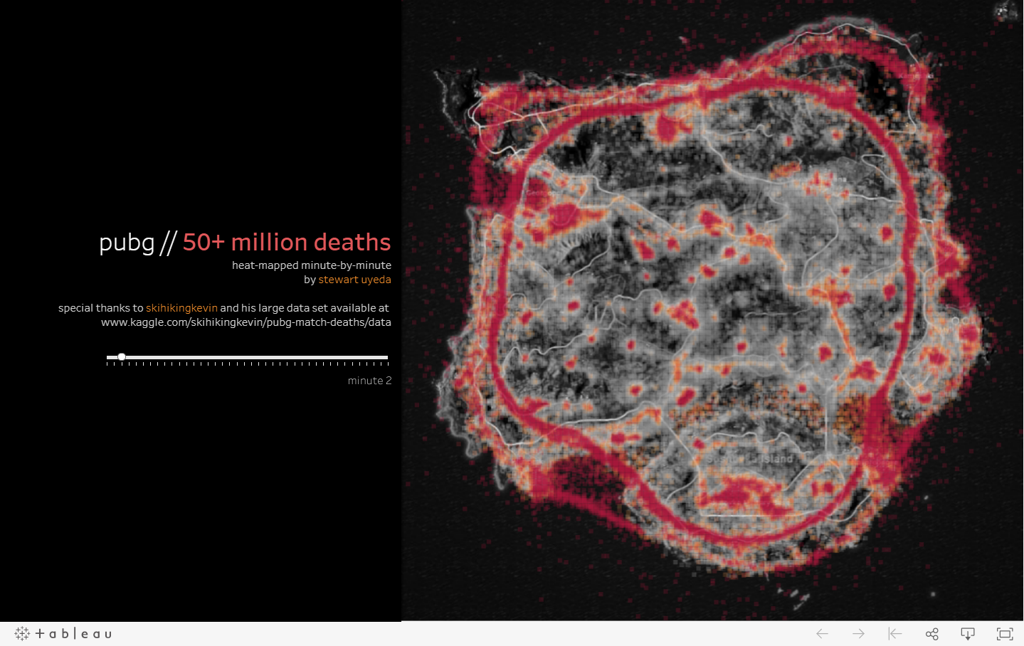
Outlink to other materials: there are also many other PUBG exploratory analysis mostly about the geographic mapping of combat location (using killer_position and victim_position) to the game maps. Among those materials, my favorite one is create by Stewart Uyeda (thank you for such amazing visualization!) and I will also post the rest with their source below.
1. By Stewart Uyeda https://public.tableau.com/profile/stewart.uyeda#!/vizhome/pubg50mildeathmap/pubg50mildeathmap Despite the masterpiece, given too much data points there is little interactive part for this Tableau.
Linear Regression on Average Player Damage vs. Average Survival Time (Answer to Problem 2)
In order to answer "On average, how many player do we eliminate before making Top10?", my first intuition would be to draw a scatter plot to visualize the related variables: Average Player Damage (100 points when eliminate a full HP player) vs. Average Survival Time (in seconds). Given that we have different game mode (solo, duo, squad) and 2 optional maps, we should draw 3 * 2 = 6 different graphs, and here is how ggplot comes into play.

ggplot not only is a great tool for scientific figures, but also it embeds statistical model to allow you build and visualize models easily. In the following figure I create a regression line for each of the 6 groups.
Although the linear regression model on average accounts for around 15% of the variance (look at r^2), here is how I address the problem:
For example in Solo mode and in map MIRAMAR, if we want to calculate on average how many playered should we eliminate to get into Top 10, we first calculate the average survival time (as x)for a player to be the 10th in rank.
df = df_PUBG %>% filter(map == "MIRAMAR", party_size == 1, team_placement == 10) %>% select(player_survive_time)
df$player_survive_time %>% mean()
# [1] 1529.484
Then we input the x into the formula and get the return value y (as avg_player_dmg)
1529.484 * 0.134 + 107
# [1] 311.9509
Since each 100 points represents a full HP player, we divide that by 100 and get
# 3.12So, on average we need to eliminate 3.12 player in order to get into Top10.
Model Selection & Parameter Tuning (Answer to Problem 3: Prediction)
Now comes the fun part, I'd like to trian a bunch of Machine Learning models to see the prediction power on getting Top10 in PUBG.
For simplicity and maximizing the signal, I choose map "MIRAMAR" and mode "Solo". MIRAMAR is the oldest map in PUBG hence contain most of our data points, while solo is chosen because situation would be more complicated when in team model (e.g. you did nothing with tier 1 teammates and you got the chicken without any action), which is what we want to avoid.
This is a classification problem with "Top10 or Not" as our response varible, with other numeric variables such as player_dbno, player_assist and distance_walk.
6 candidate classifier are chosen and R caret package is used for hyperparameter tuning and prediction; R Shiny + AWS-EC2 is used for interative classifier online, check here for the R Shiny APP. All the codes can be found in the corresponding Code Portfolio
Below is the model prediction comparison based on Accuracy and Kappa value. All the models render a high accuracy >90%.

If we plot the variable importance map for Random Forest, we can see player_survive_time is the most important features *(quantified as each mean decrease in Gini impurity / MAX(mean decrease in Gini impurity) 100, so that the maximum value will be 100)**

This makes sense because for the majority of the players, if your shooting skills is not that talented, then you might try to find a way to prolong your survival time, either by crawling on the ground or hiding in the toilet Lol.
Then I picked 3 of the models into my RShiny APP (Gradient Boosting Machine, Random Forest and Linear Discriminant Analysis).
App Address: http://ec2-52-207-221-28.compute-1.amazonaws.com:3838/myapp/
Please open from computer browser
The APP looks like this:

I strongly recommend you to open this APP from you computer browser because the mobile end or embedded browser in your social APP will mess it up.
There is user input slider panel on the left and model prediction panel on the right. You can find the predicted probability on the right bottom table column Prob.
In the second tab, I map the most important player_survival_time variable along with the probabiltiy, so that you can see how each model treat with the probability change differently given your current attributes.

Feel free to make changes to the user input panel and see how the curve changes while you change them!
App Address: http://ec2-52-207-221-28.compute-1.amazonaws.com:3838/myapp/
Please open from computer browser
Conclusion and Acknowledgement
It's been nearly a month since I first came up with this project and finally it is reaching a happy ending. The data collection and processing procedure is rewinding and torturing but I truly value the training and exploring. From my point of view, the most valuable thing about a data scientist is his experience and insight about data and values: How to select features and do feature engineering? How to maximize signals? How to tuning and select models? Indeed this requires a lot of knowledge either from Math, Stat, CS and even other domain, but one good thing about data science is that: you never get bored!
Thanks a lot to Sherlley for supporing my interests and career even if that means I need to stay up late many many times. Thanks a lot to my friends and family who take a valuable part of their life viewing my work and ideas. Last thank to myself, you've walked a long way and thank you for persevering and never giving up!
Ancheng (Maximus)
Sep 11, 2018