
Project Description
Abstract
Traffic is among the biggest causes of injuries or deaths in today’s mega cities. With Google map, people are feeling more convenient travelling but not more secured, for that there hasn’t been one product that can alert people about potential traffic accidents on streets they are driving through. Now I'd like to propose a Traffic Warning System to help predict on the potential risk of traffic accident in streets of Brooklyn, New York.
I collected datasets from Google Bigquery Public Dataset and NYC Open Data Website. Generalized Linear Mixed Effect Model is considered for predicting the probability of traffic accidents based on time, traffic speed, weather, road construction and 311 service report. After evaluating the result of preliminary GLM model, I find speed to be insignificant to the model, while weather condition is of much significance in predicting occurrence of traffic accidents. With the final model I obtain 21.3% power with about 10% type I error rate on predicting occurrence of traffic accidents on 1023 streets of Brooklyn in testing set.
Introduction
Domain Problem
New York City Council passed a local law in 2011 that allows the collection and publication of NYC traffic collision data, which enables researchers to study the temperal and spatial information of the traffic accidents. Based upon this data, I'd like to consider using GLMM models I learnt from class to perform on such datasets and see whether it can be used for real-life purpose.
The collision datset itself is not adequate for building the model. After searching throughout the internet for other available metrices, I found the other datasets: NYC road construction record, NYC 311 service log and historical weather in Brooklyn. These datasets are useful because they directly relate to traffic conditions and they contains time and location information, i.e. can be matched to the traffic collision dataset.
Given the time and range of this paper, I filter the collision dataset from 2017-03-01 to 2018-01-21. The reason for the end date of dataset is due to both the incomplete dataset from Google Bigquery (they claim that the data is up-to-date but in fact it is not) and the intersection of multiple datasets (I want most of observations contained all the metrices). Finally the cleaned dataset contain 25796 observations with 51 variables.
Exploratory Analysis
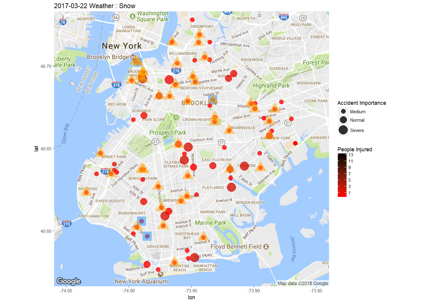
First I'd like to explore where does those traffic collision happened. Both point map and density map are performed to visulize the accident in Brooklyn borough. In order the draw the density map, I use cumulative dataset to better show the trend of the collision cumulation as well as better pinpoint the hot zone of traffic collision. Sample Collision Information Map on 2017-3-22 indicates the accident importance and number of people injured in the traffic accidents happen on a single day of Mar22 2017. Note that the weather condition is snow, which I'll show later to be a significant factor to traffic accidents.

The Dynamic Density Map of Cumulative Collisions till 2018-01-21 shows the cumulative collision density from 2017-03-01 to 2018-01-21. Note that from top to bottom, Williamsburg, Altantic Avenue and Flatbush Avenue are among the highest frequency of collision accidents.

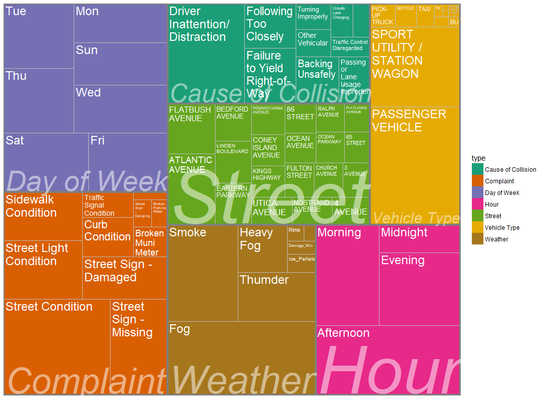
Next I want to visualize the contributing factors by their appearing frequency in the collision. I use Treemaps and select contributing factors of interests: Day of Week, Hour, 311 Service Complaint Type, etc.. From the treemap we can see that the previously mentioned Altantic Avenue and Flatbush Avenue are truly the most dangerous streets in Brooklyn. We can also notice that the main reason for accidents is Driver Inattention/Distraction, and the government should consider putting more emphasis on noticing people about its danger. In terms of weather condition, most accident happened when the weather is Fog or Smoke.

Methods
Data Collection & Manipulation
In order to perform the analysis, I have to merge the collision, weather, construction information, 311 service log and speed dataset together as a single dataframe. I first downloaded the whole dataset of all metrices, each in different excel sheets. I uniform the time variable in each sheet to POSIXct (timezone = EST) and filter the dataset by time range from 2017-03-01 to 2018-01-22. Next is merging the events of collision with the metrices at the same location. I utilize the geological information (longitude and latitude) for spatial matching with precision of about 300 meters in radius. The speed datasets consists of speed information from all traffic cameras with speed detector in NYC and is recorded every 5 minutes. The speed data is stored in large excel sheets and I manage to filter them by Brooklyn borough and merge together as a single excel sheet. The ultimate speed dataset contains speed data from 18 speed detector in Brooklyn. I first match the street of collision with the camera unique linkid, then match the time within 10 minutes of the accident (use average speed). The other metrices are matched to collision events in the same way. Given the relative small amount of available speed camera in Brooklyn, the ultimate model dataset with speed information narrows down to 304 observations with 7 linkid (i.e. 7 street levels).
Preliminary Model
The model to my instinct is the one-level Generalized Linear Mixed Effect Model (GLMM):
\(
\begin{aligned}
logit(E[y_{ij}|\mu_i]) = \beta_0 &+ u_i + \beta_1*Speed_{ij} + \beta_{2}*1\{Time_{ij} = Morning\} + \beta_{3}*1\{Time_{ij} = Afternoon\} \\
&+ \beta_{4}*1\{Time_{ij} = Night\} + \beta_{5}*1\{Time_{ij} = Midnight\} + \beta_6*Rainfall_{ij}\\
& + \beta_7*Snowdepth_{ij} + \beta_{8}*1\{Weather\ Type_{ij}=Fog\}+ \beta_{9}*1\{Weather\ Type_{ij}=Thunder\} \\
&+ \beta_{10}*1\{Weather\ Type_{ij}=Smoke\}+ \beta_{11}*1\{Weather\ Type_{ij}=Ice Pellet\}\\
& + \beta_{12}*1\{Roadwork_{ij}=True\} + \beta_{13}*1\{311Service_{ij}=True\}
\end{aligned}
\)
\(
i:\ street,\ \ j:\ accident\ at\ street\ i,\ u_i\sim N(0, \sigma^2)
\)
\(
\begin{aligned}
y_{ij} &= 1,\ if\ accident\ j\ caused\ by\ nondriver\ factors\ happens\ at\ street\ i\\
y_{ij} &= 0,\ otherwise
\end{aligned}
\)
Then I stratified-split the dataset by ratio of 8:2, write the formula into glmer() to fit on training set and see the result:
Generalized linear mixed model fit by maximum likelihood (Adaptive Gauss-Hermite Quadrature, nAGQ = 50) ['glmerMod']
 Family: binomial  ( logit )
Formula: y ~ speed + factor(hour_div) + RainFall + SnowDepth + Fog + Thumder +
    Smoke + Ice_Pellets + (Construction == "Yes") + call4road +      (1 | linkid)
   Data: df_train
Control: glmerControl(optimizer = "bobyqa")

     AIC      BIC   logLik deviance df.resid
   352.7    401.6   -162.3    324.7      229

Scaled residuals:
       Min         1Q     Median         3Q        Max
-1.9268315 -0.9206406 -0.6487477  1.0131595  1.4761933

Random effects:
 Groups Name        Variance Std.Dev.
 linkid (Intercept) 0        0
Number of obs: 243, groups:  linkid, 7

Fixed effects:
                              Estimate   Std. Error  z value Pr(>|z|)
(Intercept)               -0.098198586  0.411153523 -0.23884 0.811232
speed                      0.007086588  0.008555082  0.82835 0.407473
factor(hour_div)Midnight   0.246678600  0.539778893  0.45700 0.647672
factor(hour_div)Morning   -0.062978348  0.302321136 -0.20832 0.834982
factor(hour_div)Night      0.047951092  0.448991589  0.10680 0.914950
RainFall                   1.985541626  0.957263614  2.07418 0.038062 *
SnowDepth                  0.187680034  0.172223470  1.08975 0.275825
FogTRUE                   -0.230906735  0.309801201 -0.74534 0.456067
ThumderTRUE               -0.481695638  0.385351257 -1.25002 0.211293
SmokeTRUE                 -0.078852210  0.298247460 -0.26439 0.791483
Ice_PelletsTRUE            0.246364007  0.772278225  0.31901 0.749719
Construction == "Yes"TRUE  0.964580224  1.235333665  0.78083 0.434905
call4roadTRUE             -0.305557640  0.280056232 -1.09106 0.275247
---
Signif. codes:  0 ‘***’ 0.001 ‘**’ 0.01 ‘*’ 0.05 ‘.’ 0.1 ‘ ’ 1
Note from the p-value of the fixed effect that except for RainFall, none of the factors are significant. Especially, the estimated coefficient for speed is 0.007, almost no effect on the model. In addition, the estimated variance for random effect is 0, which means that there are no random street level effect, and that is clearly not what I expect.
One thing worthy of further discussion is the insignificant effect of speed. Our instinct tells us that the higher speed will leave shorter reaction time to change of traffic condition, hence will be a major effect in predicting collision. However, the model tells the opposite, of which the weather condition (such as RainFall in mm unit) plays a much more important part. Possible reasons for this is:
There are only 7 speed camera data in our training model, and they are distributed mostly in the 278 express way and around the Red Hook and Greenpoint region (please see the camera distribution map below). Given the limitation of the camera location, speed on the road is reasonably not very significant. For example, in the express way, traffic speed is indeed high but also large gap between vehicles, hence drivers could have equal amount of time to respond to sudden change of traffic and will not be significantly more dangerous with a higher speed.
The speed information is the average speed recorded by the speed camera on the road, with no direct relationship with the speed of the vehicles involved in the accident. And we know the accidents only happen in a fairly small amount of vehicles compare to the large volumn of traffic.
There may be multicollinearity in our predictors, and we should take a look.
Multicollinearity
Call:
omcdiag(x = df_vif, y = as.numeric(df_model$y))

Overall Multicollinearity Diagnostics

                       MC Results detection
Determinant |X'X|:         0.3511         0
Farrar Chi-Square:       314.6253         1
Red Indicator:             0.1253         0
Sum of Lambda Inverse:    14.2751         0
Theil's Method:            1.4489         1
Condition Number:          8.3896         0

1 --> COLLINEARITY is detected by the test
0 --> COLLINEARITY is not detected by the test
From the result we know that the determinant is relatively small and based on the majority voting I conclude that there is more likely to be no multicollinearity within our model dataset.
Modified Model
I then decide to remove the speed variable from the dataset. By removing it I can then make use of a way larger datset (of 25796 observations) with other factors such as weather and construction. Then we also do the stratified-split of the dataset by on_street_name and further assign random intercept to each street in our one-level generalized linear mixed effect model.
\(\begin{aligned}
logit(E[y_{ij}|\mu_i]) = \beta_0 &+ u_i + \beta_{1}*1\{Time_{ij} = Morning\} + \beta_{2}*1\{Time_{ij} = Afternoon\} + \beta_{3}*1\{Time_{ij} = Night\} \\
&+ \beta_{4}*1\{Time_{ij} = Midnight\} + \beta_5*Rainfall_{ij} + \beta_6*Snowdepth_{ij} + \beta_{7}*1\{Weather\ Type_{ij}=Fog\}\\
&+ \beta_{8}*1\{Weather\ Type_{ij}=Thunder\} + \beta_{9}*1\{Weather\ Type_{ij}=Smoke\}\\
&+ \beta_{10}*1\{Weather\ Type_{ij}=Ice Pellet\} + \beta_{11}*1\{Roadwork_{ij}=True\} \\
&+ \beta_{12}*1\{311Service_{ij}=True\}
\end{aligned}
\)
And apply the GLM model:
Generalized linear mixed model fit by maximum likelihood (Adaptive Gauss-Hermite Quadrature, nAGQ = 50) ['glmerMod']
 Family: binomial  ( logit )
Formula: y ~ factor(hour_div) + RainFall + SnowDepth + Fog + Thumder +      Smoke + Ice_Pellets + (Construction == "Yes") + call4road +
    (1 | on_street_name)
   Data: df_train
Control: glmerControl(optimizer = "bobyqa")

     AIC      BIC   logLik deviance df.resid
 29871.5  29976.3 -14922.8  29845.5    23294

Scaled residuals:
       Min         1Q     Median         3Q        Max
-1.4545914 -0.7893971 -0.5833948  1.1017576  2.0418863

Random effects:
 Groups         Name        Variance  Std.Dev.
 on_street_name (Intercept) 0.1436875 0.3790614
Number of obs: 23307, groups:  on_street_name, 1023

Fixed effects:
                              Estimate   Std. Error  z value   Pr(>|z|)
(Intercept)               -0.352620101  0.039628157 -8.89822 < 2.22e-16 ***
factor(hour_div)Midnight  -0.189438446  0.048541798 -3.90258 9.5171e-05 ***
factor(hour_div)Morning   -0.107810768  0.033677525 -3.20127 0.00136824 **
factor(hour_div)Night      0.012758000  0.039408976  0.32373 0.74613992
RainFall                  -0.018646139  0.050830662 -0.36683 0.71374689
SnowDepth                  0.066616718  0.013212039  5.04212 4.6040e-07 ***
FogTRUE                    0.121616365  0.032064870  3.79282 0.00014894 ***
ThumderTRUE               -0.010666984  0.038142516 -0.27966 0.77973740
SmokeTRUE                  0.073333952  0.031371865  2.33757 0.01940953 *
Ice_PelletsTRUE           -0.283226486  0.099584507 -2.84408 0.00445396 **
Construction == "Yes"TRUE -0.185226448  0.092260275 -2.00765 0.04468037 *
call4roadTRUE              0.002981955  0.029691397  0.10043 0.92000167
---
Signif. codes:  0 ‘***’ 0.001 ‘**’ 0.01 ‘*’ 0.05 ‘.’ 0.1 ‘ ’ 1

Correlation of Fixed Effects:
              (Intr) fctr(hr_dv)Md fctr(hr_dv)Mr fc(_)N RanFll SnwDpt FgTRUE ThTRUE SmTRUE I_PTRU C=="Y"
fctr(hr_dv)Md -0.237
fctr(hr_dv)Mr -0.356  0.286
fctr(hr_d)N   -0.297  0.247         0.351
RainFall       0.020 -0.009         0.004        -0.003
SnowDepth     -0.146  0.012         0.003         0.009 -0.048
FogTRUE       -0.279 -0.003        -0.005        -0.003 -0.327  0.072
ThumderTRUE   -0.053  0.011         0.006        -0.002 -0.189  0.053 -0.159
SmokeTRUE     -0.127  0.003        -0.002        -0.001  0.028 -0.093 -0.260 -0.030
Ic_PlltTRUE    0.026 -0.007        -0.004        -0.009 -0.051 -0.380 -0.070  0.008 -0.068
C=="Ys"TRUE   -0.094  0.007         0.011         0.017 -0.005  0.016 -0.008 -0.011  0.002 -0.001
call4rdTRUE   -0.461 -0.004        -0.001        -0.003 -0.017  0.102 -0.006 -0.046 -0.007  0.014 -0.013
Note from the result that now I obtained a lot significant coefficient values than the previous model by removing the speed variable. Among the variables, hours, weather conditions like SnowDepth and Fog have the most significant coefficients, and the coefficient for whether there is a construction on going in the street is also statistically significant. The result correspond with my assumption that the traffic accident that are caused by non-driver factors comes from bad weather conditions and roadworks. From the result, the 311 service call related to road conditions doesn't seems to be related to the accidents, although such calls are made before accidents happen.
Next, I'd like to know if we are legitimate to remove those variables with non-significant coefficients. Wald's Test is used to perform the hypothesis testing.
Wald's Test
The null hypothesis is that there are no difference between my current model and a simplified version. \(\beta_5\), \(\beta_8\) and \(\beta_{12}\) represent coefficients for RainFall, Thunder and 311 Service Call respectively.
\(H_0:\ \beta_5=\beta_8=\beta_{12}=0
\)
summary_mod2 <- summary(mod.2)
L <- matrix(0, nrow = 3, ncol = 12)
L[1,5] <- L[2,8] <- L[3,12] <- 1

Fstar <- t(L %*% summary_mod2$coefficients[,1]) %*%
  solve(L %*% summary(mod.2)$vcov %*% t(L)) %*%
  (L %*% summary_mod2$coefficients[,1])

pchisq(as.numeric(Fstar), df = 3, lower.tail = FALSE)

          [,1]
[1,] 0.9661755
The return value is the p-value for the Wald's Test, and p-value >> 0.05 tells I am legitimate to remove the RainFall, Thunder and 311 Service Call from my model at the same time, i.e. I fail to reject the null hypothesis that those coefficients are all equal to 0.
Final Model
In my final model, I take the remain variables from the last step and am ready to test my model on the testing dataset.
\(
\begin{aligned}
logit(E[y_{ij}|\mu_i]) = \beta_0 &+ u_i + \beta_{1}*1\{Time_{ij} = Morning\} + \beta_{2}*1\{Time_{ij} = Afternoon\} + \beta_{3}*1\{Time_{ij} = Night\} \\
&+ \beta_{4}*1\{Time_{ij} = Midnight\} + \beta_5*Snowdepth_{ij} + \beta_6*1\{Weather\ Type_{ij}=Fog\}\\
&+ \beta_{7}*1\{Weather\ Type_{ij}=Smoke\} + \beta_{8}*1\{Weather\ Type_{ij}=Ice Pellet\}\\
&+ \beta_{9}*1\{Roadwork_{ij}=True\}
\end{aligned}
\)
and have
Generalized linear mixed model fit by maximum likelihood (Adaptive Gauss-Hermite
  Quadrature, nAGQ = 50) [glmerMod]
 Family: binomial  ( logit )
Formula: y ~ factor(hour_div) + SnowDepth + Fog + Smoke + Ice_Pellets +
    (Construction == "Yes") + (1 | on_street_name)
   Data: df_train
Control: glmerControl(optimizer = "bobyqa")

     AIC      BIC   logLik deviance df.resid
 29865.8  29946.4 -14922.9  29845.8    23297

Scaled residuals:
    Min      1Q  Median      3Q     Max
-1.4560 -0.7903 -0.5828  1.1011  2.0478

Random effects:
 Groups         Name        Variance Std.Dev.
 on_street_name (Intercept) 0.1435   0.3788
Number of obs: 23307, groups:  on_street_name, 1023

Fixed effects:
                          Estimate Std. Error z value Pr(>|z|)
(Intercept)               -0.35163    0.03504 -10.035  < 2e-16 ***
factor(hour_div)Midnight  -0.18943    0.04854  -3.903 9.51e-05 ***
factor(hour_div)Morning   -0.10768    0.03368  -3.198  0.00139 **
factor(hour_div)Night      0.01269    0.03941   0.322  0.74738
SnowDepth                  0.06649    0.01311   5.070 3.97e-07 ***
FogTRUE                    0.11527    0.02943   3.916 8.98e-05 ***
SmokeTRUE                  0.07339    0.03135   2.341  0.01923 *
Ice_PelletsTRUE           -0.28526    0.09949  -2.867  0.00414 **
Construction == "Yes"TRUE -0.18569    0.09223  -2.013  0.04409 *
---
Signif. codes:  0 ‘***’ 0.001 ‘**’ 0.01 ‘*’ 0.05 ‘.’ 0.1 ‘ ’ 1

Correlation of Fixed Effects:
              (Intr) fctr(hr_dv)Md fctr(hr_dv)Mr fc(_)N SnwDpt FgTRUE SmTRUE I_PTRU
fctr(hr_dv)Md -0.269
fctr(hr_dv)Mr -0.403  0.286
fctr(hr_d)N   -0.337  0.247         0.351
SnowDepth     -0.108  0.012         0.003         0.010
FogTRUE       -0.363 -0.004        -0.002        -0.005  0.075
SmokeTRUE     -0.149  0.004        -0.001        -0.001 -0.090 -0.280
Ic_PlltTRUE    0.037 -0.008        -0.004        -0.009 -0.388 -0.094 -0.067
C=="Ys"TRUE   -0.114  0.007         0.011         0.017  0.018 -0.014  0.002 -0.001
Now all the coefficients are significant, we can now move on to evaluate the predicting quality of our GLMM model.
Prediction Results
Prediction on Testing Set
First we plot the response vs. link under the Training Set in order to find the decision threshold. The red points is where \(y_{ij}=1\) and black is where \(y{ij}=0\). Some of the red and black points mix together but there is still a noticable trend that when response > 0.47, red points are the majority.

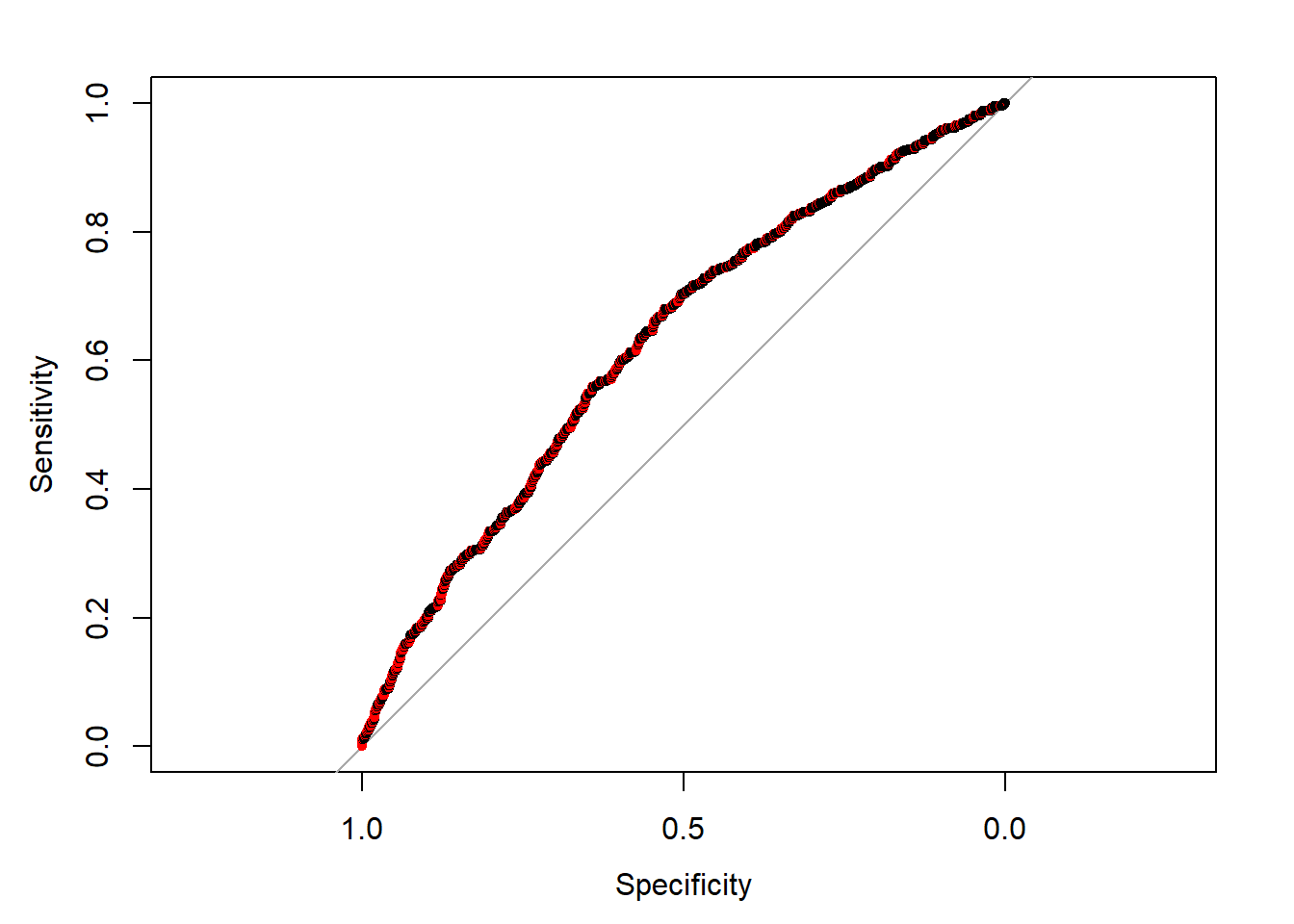
Another way to evaluate the binary classfier is the ROC curve. Note that the AUC (area under the curve) is 0.6268.

As mentioned before, we can take the classfication threhold = 0.47 as decision criteria. And using this threshold we are able to evaluate the prediction on our testing set.
# prediction on df_test
y_pred = predict(mod.2, newdata = df_test, type = "response") > 0.47 # decision criteria
(tab_eval = table(y_pred, df_test$y))
##
## y_pred FALSE TRUE
## FALSE 1371 731
## TRUE 183 204

(alpha = tab_eval[2]/(tab_eval[1] + tab_eval[2]))
## [1] 0.1177606
(power = tab_eval[4]/(tab_eval[3] + tab_eval[4]))
## [1] 0.2181818
Note from the table, when the Type I Error $\alpha$ is set to be around 10%, then the power of the model is about 22%, i.e. in every 5 car accidents that are caused by non-driver factors, then the model can successfully predict one.
Discussion
There are both important findings and things to improve in my model. One of the most important thing I learn from the model is that on the contrary of what I expected, the speed is not a significant factor in the model. One thing need to be emphasized is that the speed data I use is not the speed of the vehicle involved in the accident but the speed of the street when the accident happens. It's very likely that the vehicles that are caught into accident are those outliers from the average speed of the street.
My model is trying to predict the probabiltiy that vehicles will run into a traffic accident caused mainly by non-driver factors, and the final model satisfactorily perform just as what I expect, that bad weather and road conditions will increse the probability of having an accident as well as when the time is at night.
In order to improve the model, the best way is to find more non-driver data related to the accident or the driver information, using which I can further distinguish the non-driver factor accidents from the accidents that are directly caused by misbehavior of the driver. In reality, most of the accidents nowadays are caused by driver-related issues, and my model prediction performance has its natural limitation.